Assessing Read Quality

Overview

Teaching: 30 min
Exercises: 15 min

Questions

How can I describe the quality of my data?

Objectives

Explain how a FASTQ file encodes per-base quality scores.

Interpret a FastQC plot summarizing per-base quality across all reads.

Bioinformatic workflows

When working with high-throughput sequencing data, the raw reads you get off of the sequencer will need to pass through a number of different tools in order to generate your final desired output. The execution of this set of tools in a specified order is commonly referred to as a workflow or a pipeline.

An example of the workflow we will be using for our variant calling analysis is provided below with a brief description of each step.

workflow

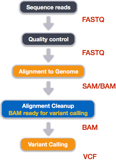
Quality control - Assessing quality using FastQC
Quality control - Trimming and/or filtering reads (if necessary)
Align reads to reference genome
Perform post-alignment clean-up
Variant calling

These workflows in bioinformatics adopt a plug-and-play approach in that the output of one tool can be easily used as input to another tool without any extensive configuration. Having standards for data formats is what makes this feasible. Standards ensure that data is stored in a way that is generally accepted and agreed upon within the community. The tools that are used to analyze data at different stages of the workflow are therefore built under the assumption that the data will be provided in a specific format.

Starting with Data

Often times, the first step in a bioinformatic workflow is getting the data you want to work with onto a computer where you can work with it. If you have outsourced sequencing of your data, the sequencing center will usually provide you with a link that you can use to download your data. Today we will be working with publicly available sequencing data.

We are studying a subset of 1000 genomes data that have been reduced in size to help the workshop run more efficiently. The data have been copied to a shared folder that you all have access.

To download the data, run the commands below.

Here we are using the -p option for mkdir. This option allows mkdir to create the new directory, even if one of the parent directories doesn’t already exist. It also suppresses errors if the directory already exists, without overwriting that directory.

mkdir -p ~/dc_workshop/data/untrimmed_fastq/
cd ~/dc_workshop/data/untrimmed_fastq

cp /mnt/shared/1000_genomes_subset/NA12873_R1.fq.gz .
cp /mnt/shared/1000_genomes_subset/NA12873_R2.fq.gz .
cp /mnt/shared/1000_genomes_subset/NA12874_R1.fq.gz .
cp /mnt/shared/1000_genomes_subset/NA12874_R2.fq.gz .
cp /mnt/shared/1000_genomes_subset/NA12878_R1.fq.gz .
cp /mnt/shared/1000_genomes_subset/NA12878_R2.fq.gz .

Faster option

If that seems like a lot of typing, so you can use “wild-cards” as we have seen previously to copy everything in one go
$ cp /mnt/shared/1000_genomes_subset/*.fq.gz .
This command creates a copy of each of the files in the /mnt/shared/1000_genomes_subset directory that end in fq.gz and places the copies in the current working directory (signified by .).

File extensions

The files we are processing are known as “fastq”, but as we mentioned previously command-line systems are not fussy about what extension a particular file has. The files in our dataset all end .fq.gz, but you might come across files that end in .fastq.gz. It shouldn’t matter to the software you use, so long as they contents are laid out (formatted) according to the same specification.

Checking the file transfer with md5sums

When moving or copying large files around, it would be wise to check that the file transfer was successful. A common way of doing this is to compute a checksum for each of the files. A checksum is

“a small-size datum from a block of digital data for the purpose of detecting errors which may have been introduced during its transmission or storage”

You can think of it as a digital fingerprint of a file, and if the contents of the file are changed in any way, a different checksum will be generated. The person making files available to you will often generate a checksum on their system and make the results available. Here, we look at the checksums generated for the example dataset and make a copy.

$ cp /mnt/shared/1000_genomes_subset/md5sums.txt .
$ cat md5sums.txt

We can re-generate the checksums and if they agree

$ md5sum NA12873_R2.fq.gz
$ md5sum -c md5sums.txt

The data comes in a compressed format, which is why there is a .gz at the end of the file names. This makes it faster to transfer, and allows it to take up less space on our computer. Let’s unzip one of the files so that we can look at the fastq format.

$ gunzip NA12873_R1.fq.gz

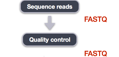
Quality Control

We will now assess the quality of the sequence reads contained in our fastq files.

workflow_qc

Details on the FASTQ format

Although it looks complicated (and it is), we can understand the fastq format with a little decoding. Some rules about the format include…

Line	Description
1	Always begins with ‘@’ and then information about the read
2	The actual DNA sequence
3	Always begins with a ‘+’ and sometimes the same info in line 1
4	Has a string of characters which represent the quality scores; must have same number of characters as line 2

We can view the first complete read in one of the files our dataset by using head to look at the first four lines.

$ head -n 4 NA12873_R1.fq

@SRR768307.13/1
AGCCCTCACAGGAGGCAAGATTGGGTTCTGGGCTGGCATTTGATGGAGGAAGCCTGGATAGTTTCTCTTGCTATCAGCGGGCAGCAGCTGGAAGGAAATGT
+
2KJBEHFFEEDG@DGHCCEDGGABFFGHEHIGHEDGBGGFHIFFEHFHC5DHIIKJLHIIGBDFGKIHDGKJ<GEL>J@HHCAKJKIEFEKH=FEE#####

Line 4 shows the quality for each nucleotide in the read. Quality is interpreted as the probability of an incorrect base call (e.g. 1 in 10) or, equivalently, the base call accuracy (e.g. 90%). To make it possible to line up each individual nucleotide with its quality score, the numerical score is converted into a code where each individual character represents the numerical quality score for an individual nucleotide. For example, in the line above, the quality score line is:

2KJBEHFFEEDG@DGHCCEDGGABFFGHEHIGHEDGBGGFHIFFEHFHC5DHIIKJLHIIGBDFGKIHDGKJ<GEL>J@HHCAKJKIEFEKH=FEE#####

The numerical value assigned to each of these characters depends on the sequencing platform that generated the reads. The sequencing machine used to generate our data uses the standard Sanger quality PHRED score encoding, using Illumina version 1.8 onwards. Each character is assigned a quality score between 0 and 41 as shown in the chart below.

Quality encoding: !"#$%&'()*+,-./0123456789:;<=>?@ABCDEFGHIJ
                   |         |         |         |         |
Quality score:    01........11........21........31........41                                

Each quality score represents the probability that the corresponding nucleotide call is incorrect. This quality score is logarithmically based, so a quality score of 10 reflects a base call accuracy of 90%, but a quality score of 20 reflects a base call accuracy of 99%. These probability values are the results from the base calling algorithm and depend on how much signal was captured for the base incorporation.

Looking back at our read:

@SRR768307.13/1
AGCCCTCACAGGAGGCAAGATTGGGTTCTGGGCTGGCATTTGATGGAGGAAGCCTGGATAGTTTCTCTTGCTATCAGCGGGCAGCAGCTGGAAGGAAATGT
+
2KJBEHFFEEDG@DGHCCEDGGABFFGHEHIGHEDGBGGFHIFFEHFHC5DHIIKJLHIIGBDFGKIHDGKJ<GEL>J@HHCAKJKIEFEKH=FEE#####

we can now see that there is a range of quality scores, but that the end of the sequence is very poor (# = a quality score of 2).

Exercise

What is the last read in the NA12873_R1.fq file? How confident are you in this read?
Solution
$ tail -n 4 NA12873_R1.fq 
@SRR768307.1457842/1
TTTATATAATTAATGTCCAATATTGCAAAGCTGTCATTACTGTCATTTTCATTAATAACTTATTATATGATTAATAATTGCATAATTAATAATGCATTTAT
+
2II?FCGCGFFDHGHGIHHJGFHGGJIKLKHJIIJIIHGIKJIKJIIIIJIJIHNKHNJLJIKJIKIKLKKJINJILKHLKIIFHECAE@9?<AC@@;;6C
This read has more consistent quality at its end than the first read that we looked at, but still has a range of quality scores, most of them high. We will look at variations in position-based quality in just a moment.

Assessing Quality using FastQC

In real life, you won’t be assessing the quality of your reads by visually inspecting your fastq files. Rather, you’ll be using software programs to assess read quality and filter out poor quality reads. We’ll first use a program called FastQC to visualize the quality of our reads. Later in our workflow, we’ll use another program to filter out poor quality reads.

At this point, lets validate that all the relevant tools are installed. If you are using the cluster-in-the-cloud then these should be preinstalled.

$ module avail

---------------------------------------------------------------- /mnt/shared/modules/all ----------------------------------------------------------------
   Autoconf/2.69-GCCcore-10.2.0                  Perl/5.32.0-GCCcore-10.2.0                    gompi/2020b
   Automake/1.16.2-GCCcore-10.2.0                Pillow/8.0.1-GCCcore-10.2.0                   gperf/3.1-GCCcore-10.2.0
   Autotools/20200321-GCCcore-10.2.0             PyYAML/5.3.1-GCCcore-10.2.0                   groff/1.22.4-GCCcore-10.2.0
   BCFtools/1.12-GCC-10.2.0                      Python/2.7.18-GCCcore-10.2.0                  help2man/1.47.4
   BWA/0.7.17-GCC-10.2.0                         Python/3.8.6-GCCcore-10.2.0            (D)    help2man/1.47.16-GCCcore-10.2.0    (D)
   Bison/3.5.3                                   SAMtools/1.12-GCC-10.2.0                      hwloc/2.2.0-GCCcore-10.2.0
   Bison/3.7.1-GCCcore-10.2.0                    SQLite/3.33.0-GCCcore-10.2.0                  hypothesis/5.41.2-GCCcore-10.2.0
   Bison/3.7.1                         (D)       ScaLAPACK/2.1.0-gompi-2020b                   intltool/0.51.0-GCCcore-10.2.0
   CMake/3.18.4-GCCcore-10.2.0                   SciPy-bundle/2020.11-foss-2020b               libarchive/3.4.3-GCCcore-10.2.0
   DB/18.1.40-GCCcore-10.2.0                     Tcl/8.6.10-GCCcore-10.2.0                     libevent/2.1.12-GCCcore-10.2.0
   Eigen/3.3.8-GCCcore-10.2.0                    Tk/8.6.10-GCCcore-10.2.0                      libfabric/1.11.0-GCCcore-10.2.0
   FFTW/3.3.8-gompi-2020b                        Tkinter/3.8.6-GCCcore-10.2.0                  libffi/3.3-GCCcore-10.2.0
   FastQC/0.11.9-Java-11               (L)       Trimmomatic/0.39-Java-11                      libjpeg-turbo/2.0.5-GCCcore-10.2.0
   GCC/10.2.0                                    UCX/1.9.0-GCCcore-10.2.0                      libpciaccess/0.16-GCCcore-10.2.0
   GCCcore/10.2.0                                UnZip/6.0-GCCcore-10.2.0                      libpng/1.6.37-GCCcore-10.2.0
   GMP/6.2.0-GCCcore-10.2.0                      VCFtools/0.1.16-GCC-10.2.0                    libreadline/8.0-GCCcore-10.2.0
   GSL/2.6-GCC-10.2.0                            X11/20201008-GCCcore-10.2.0                   libtool/2.4.6-GCCcore-10.2.0
   HTSlib/1.11-GCC-10.2.0                        XZ/5.2.5-GCCcore-10.2.0                       libxml2/2.9.10-GCCcore-10.2.0
   HTSlib/1.12-GCC-10.2.0              (D)       binutils/2.35-GCCcore-10.2.0                  libyaml/0.2.5-GCCcore-10.2.0
   IGV/2.9.4-Java-11                             binutils/2.35                          (D)    makeinfo/6.7-GCCcore-10.2.0
   Java/11.0.2                         (L,11)    bzip2/1.0.8-GCCcore-10.2.0                    matplotlib/3.3.3-foss-2020b
   LibTIFF/4.1.0-GCCcore-10.2.0                  cURL/7.72.0-GCCcore-10.2.0                    ncurses/6.2-GCCcore-10.2.0
   M4/1.4.18-GCCcore-10.2.0                      expat/2.2.9-GCCcore-10.2.0                    ncurses/6.2                        (D)
   M4/1.4.18                           (D)       flex/2.6.4-GCCcore-10.2.0                     networkx/2.5-foss-2020b
   Meson/0.55.3-GCCcore-10.2.0                   flex/2.6.4                             (D)    numactl/2.0.13-GCCcore-10.2.0
   MultiQC/1.9-foss-2020b-Python-3.8.6           fontconfig/2.13.92-GCCcore-10.2.0             pkg-config/0.29.2-GCCcore-10.2.0
   NASM/2.15.05-GCCcore-10.2.0                   foss/2020b                                    pybind11/2.6.0-GCCcore-10.2.0
   Ninja/1.10.1-GCCcore-10.2.0                   freebayes/1.3.5-GCC-10.2.0-Java-11.0.2        util-linux/2.36-GCCcore-10.2.0
   OpenBLAS/0.3.12-GCC-10.2.0                    freetype/2.10.3-GCCcore-10.2.0                xorg-macros/1.19.2-GCCcore-10.2.0
   OpenMPI/4.0.5-GCC-10.2.0                      gettext/0.21-GCCcore-10.2.0                   zlib/1.2.11-GCCcore-10.2.0
   PMIx/3.1.5-GCCcore-10.2.0                     gettext/0.21                           (D)    zlib/1.2.11                        (D)

The module relevant for QC purposes is called FastQC

module load FastQC

if FastQC is not installed then you would expect to see an error like

Lmod has detected the following error:  The following module(s) are unknown: "FastQC"

Please check the spelling or version number. Also try "module spider ..."
It is also possible your cache file is out-of-date; it may help to try:
  $ module --ignore-cache load "FastQC"

Also make sure that all modulefiles written in TCL start with the string #%Module

If this happens check with your instructor before trying to install it.

FastQC has a number of features which can give you a quick impression of any problems your data may have, so you can take these issues into consideration before moving forward with your analyses. Rather than looking at quality scores for each individual read, FastQC looks at quality collectively across all reads within a sample. The image below shows one FastQC-generated plot that indicates a very high quality sample:

good_quality

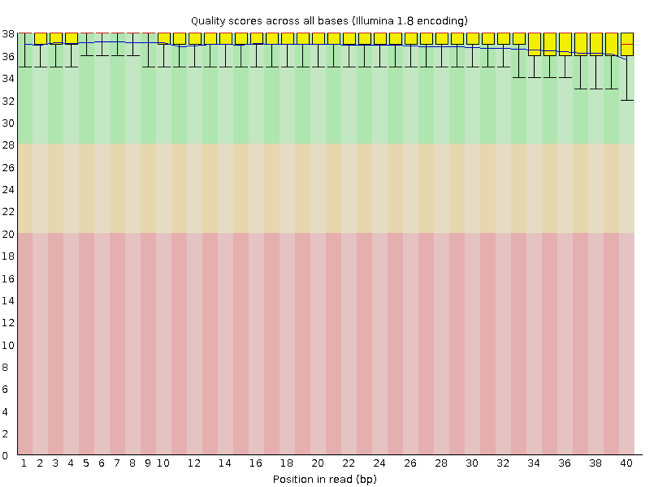
The x-axis displays the base position in the read, and the y-axis shows quality scores. In this example, the sample contains reads that are 40 bp long. This is much shorter than the reads we are working with in our workflow. For each position, there is a box-and-whisker plot showing the distribution of quality scores for all reads at that position. The horizontal red line indicates the median quality score and the yellow box shows the 1st to 3rd quartile range. This means that 50% of reads have a quality score that falls within the range of the yellow box at that position. The whiskers show the absolute range, which covers the lowest (0th quartile) to highest (4th quartile) values.

For each position in this sample, the quality values do not drop much lower than 32. This is a high quality score. The plot background is also color-coded to identify good (green), acceptable (yellow), and bad (red) quality scores.

Now let’s take a look at a quality plot on the other end of the spectrum.

bad_quality

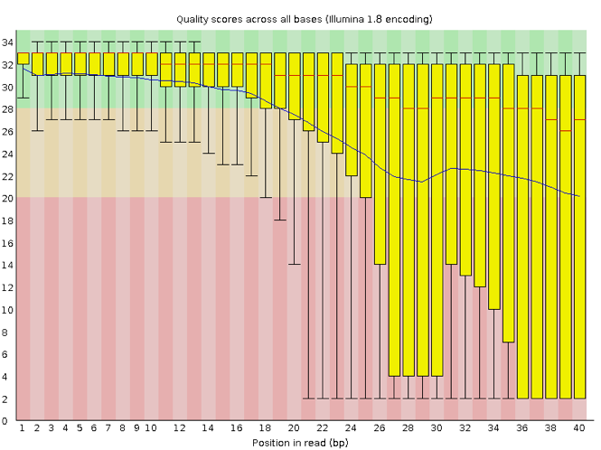
Here, we see positions within the read in which the boxes span a much wider range. Also, quality scores drop quite low into the “bad” range, particularly on the tail end of the reads. The FastQC tool produces several other diagnostic plots to assess sample quality, in addition to the one plotted above.

Input data for FastQC

FastQC doesn’t know what kind of sequencing experiment you have performed, and for this reason it is widely-used on all types of sequencing datasets (DNA-seq, RNA-seq, ChIP-seq…). You will probably come across it at some point so it worth being familiar with, even if some parts of the workshop aren’t directly applicable to your project.

Running FastQC

We will now assess the quality of the reads that we downloaded. First, make sure you’re still in the untrimmed_fastq directory

$ cd ~/dc_workshop/data/untrimmed_fastq/

The command used to run FastQC is called fastqc, and is case-sensitive. FastQC can accept multiple file names as input, and on both zipped and unzipped files, so we can use the *.fq* wildcard to run FastQC on all of the fastq files in this directory.

$ fastqc *.fq*

You will see an automatically updating output message telling you the progress of the analysis. It will start like this:

Started analysis of NA12873_R1.fq.gz
Approx 5% complete for NA12873_R1.fq.gz
Approx 10% complete for NA12873_R1.fq.gz
Approx 15% complete for NA12873_R1.fq.gz
Approx 20% complete for NA12873_R1.fq.gz

In total, it should take about one minute for FastQC to run on all our FASTQ files. When the analysis completes, your prompt will return. So your screen will look something like this:

Approx 75% complete for NA12878_R2.fq.gz
Approx 80% complete for NA12878_R2.fq.gz
Approx 85% complete for NA12878_R2.fq.gz
Approx 90% complete for NA12878_R2.fq.gz
Approx 95% complete for NA12878_R2.fq.gz
Approx 100% complete for NA12878_R2.fq.gz
Analysis complete for NA12878_R2.fq.gz
$

The FastQC program has created several new files within our data/untrimmed_fastq/ directory.

$ ls

NA12873_R1.fq           NA12874_R1_fastqc.html  NA12878_R1_fastqc.zip
NA12873_R1_fastqc.html  NA12874_R1_fastqc.zip   NA12878_R2.fq.gz
NA12873_R1_fastqc.zip   NA12874_R2.fq.gz        NA12878_R2_fastqc.html
NA12873_R2.fq.gz        NA12874_R2_fastqc.html  NA12878_R2_fastqc.zip
NA12873_R2_fastqc.html  NA12874_R2_fastqc.zip   
NA12873_R2_fastqc.zip   NA12878_R1.fq.gz
NA12874_R1.fq.gz        NA12878_R1_fastqc.html

For each input FASTQ file, FastQC has created a .zip file and a .html file. The .zip file extension indicates that this is actually a compressed set of multiple output files. The .html file is a stable webpage displaying the summary report for each of our samples.

We want to keep our data files and our results files separate, so we will move these output files into a new directory within our results/ directory.

$ mkdir -p ~/dc_workshop/results/fastqc_untrimmed_reads 
$ mv *.zip ~/dc_workshop/results/fastqc_untrimmed_reads/ 
$ mv *.html ~/dc_workshop/results/fastqc_untrimmed_reads/ 

Now we can navigate into this results directory and do some closer inspection of our output files.

$ cd ~/dc_workshop/results/fastqc_untrimmed_reads/

Combining reports

For projects involving a large number of samples, it is more convenient to consolidate all QC reports into a single page. This allows any trends and outliers to be identified more easily. A popular tool for doing this is called multiqc and can recognise the Quality Control output from a variety of tools including fastqc.

Exercise

Find and load the module that provides the multiqc tool. Consult the help page for multiqc (multiqc -h) and / or online resources to generate a combined QC report from the FastQC output that you have just generated
Solution

The multiqc tool has one compulsory argument which corresponds to the directory containing QC reports. This can be the current working directory; .
$ multiqc .

Exercise

Having FastQC write output in the current directory and move the results afterwards seems a bit cumbersome. Looking at the help for fastqc, can you see a way of specifying a different directory for the output? Delete the current contents of ~/dc_workshop/results/fastqc_untrimmed_reads/ and re-run fastqc to output files directly to this directory.
Solution

fastqc has an option -o which can be used to specify an output directory
$ rm ~/dc_workshop/results/fastqc_untrimmed_reads/*
$ ls ~/dc_workshop/results/fastqc_untrimmed_reads/ 
$ fastqc *.fq* -o ~/dc_workshop/results/fastqc_untrimmed_reads/ 
$ ls ~/dc_workshop/results/fastqc_untrimmed_reads/ 

Viewing the multiqc results

If we were working on our local computers, we’d be able to look at each of these HTML files by opening them in a web browser.

However, these files are currently sitting on our remote AWS instance, where our local computer can’t see them. And, since we are only logging into the HPC via the command line - it doesn’t have any web browser setup to display these files either.

So the easiest way to look at these webpage summary reports will be to transfer them to our local computers (i.e. your laptop).

To transfer a file from a remote server to our own machines, we will use scp, which we learned yesterday in the Shell Genomics lesson.

First we will make a new directory on our computer to store the HTML files we’re transferring. Let’s put it on our desktop for now. Open a new tab in your terminal program (you can use the pull down menu at the top of your screen or the Cmd+t keyboard shortcut) and type:

$ mkdir -p ~/Desktop/fastqc_html

Now we can transfer our HTML files to our local computer using scp.

$ scp <your_username>@ephemeron.n8cir.org.uk:~/dc_workshop/results/fastqc_untrimmed_reads/*.html ~/Desktop/fastqc_html

As a reminder, the first part of the command <your_username>@ephemeron.n8cir.org.uk is the address for your remote computer. Make sure you replace <your_username> with your username for this workshop (the one you used to log in).

The second part starts with a : and then gives the absolute path of the files you want to transfer from your remote computer. Don’t forget the :. We used a wildcard (*.html) to indicate that we want all of the HTML files.

The third part of the command gives the absolute path of the location you want to put the files. This is on your local computer and is the directory we just created ~/Desktop/fastqc_html.

You should see a status output like this:

multiqc_report.html                           100% 1164KB   1.4MB/s   00:00
NA12873_R1_fastqc.html                      100%  249KB 152.3KB/s   00:01    
NA12873_R2_fastqc.html                      100%  254KB 219.8KB/s   00:01    
NA12874_R1_fastqc.html                      100%  254KB 271.8KB/s   00:00    
NA12874_R2_fastqc.html                      100%  251KB 252.8KB/s   00:00    
NA12878_R1_fastqc.html                      100%  249KB 370.1KB/s   00:00    
NA12878_R2_fastqc.html                      100%  251KB 592.2KB/s   00:00  

Now we can go to our new directory and open the multiqc report, or the individual reports if we wish.

Depending on your system, you should be able to select and open them all at once via a right click menu in your file browser.

Exercise

Discuss your results with your breakout group. Which sample(s) looks the best in terms of per base sequence quality? Which sample(s) look the worst?

Solution

All of the reads contain usable data, but the quality decreases toward the end of the reads.

Decoding the other FastQC outputs – Optional

We’ve now looked at quite a few “Per base sequence quality” FastQC graphs, but there are nine other graphs that we haven’t talked about! Below we have provided a brief overview of interpretations for each of these plots. For more information, please see the FastQC documentation here

Per tile sequence quality: the machines that perform sequencing are divided into tiles. This plot displays patterns in base quality along these tiles. Consistently low scores are often found around the edges, but hot spots can also occur in the middle if an air bubble was introduced at some point during the run.
Per sequence quality scores: a density plot of quality for all reads at all positions. This plot shows what quality scores are most common.
Per base sequence content: plots the proportion of each base position over all of the reads. Typically, we expect to see each base roughly 25% of the time at each position, but this often fails at the beginning or end of the read due to quality or adapter content.
Per sequence GC content: a density plot of average GC content in each of the reads.
Per base N content: the percent of times that ‘N’ occurs at a position in all reads. If there is an increase at a particular position, this might indicate that something went wrong during sequencing.
Sequence Length Distribution: the distribution of sequence lengths of all reads in the file. If the data is raw, there is often on sharp peak, however if the reads have been trimmed, there may be a distribution of shorter lengths.
Sequence Duplication Levels: A distribution of duplicated sequences. In sequencing, we expect most reads to only occur once. If some sequences are occurring more than once, it might indicate enrichment bias (e.g. from PCR). If the samples are high coverage (or RNA-seq or amplicon), this might not be true.
Overrepresented sequences: A list of sequences that occur more frequently than would be expected by chance.
Adapter Content: a graph indicating where adapater sequences occur in the reads.
K-mer Content: a graph showing any sequences which may show a positional bias within the reads.

Other notes – Optional

Quality Encodings Vary

Although we’ve used a particular quality encoding system to demonstrate interpretation of read quality, different sequencing machines use different encoding systems. This means that, depending on which sequencer you use to generate your data, a # may not be an indicator of a poor quality base call.

This mainly relates to older Solexa/Illumina data, but it’s essential that you know which sequencing platform was used to generate your data, so that you can tell your quality control program which encoding to use. If you choose the wrong encoding, you run the risk of throwing away good reads or (even worse) not throwing away bad reads!

Same Symbols, Different Meanings

Here we see > being used as a shell prompt, whereas > is also used to redirect output. Similarly, $ is used as a shell prompt, but, as we saw earlier, it is also used to ask the shell to get the value of a variable.

If the shell prints > or $ then it expects you to type something, and the symbol is a prompt.

If you type > or $ yourself, it is an instruction from you that the shell should redirect output or get the value of a variable.

Key Points

Quality encodings vary across sequencing platforms.

FastQC and multiqc can generate quality control reports for sequencing data

Keep your project directories tidy

Files can be copied from HPC to your own machine for interactive visualisation

previous episode

Data Wrangling and Processing for Genomics

next episode

Assessing Read Quality

Overview

Bioinformatic workflows

Starting with Data

Faster option

File extensions

Checking the file transfer with md5sums

Quality Control

Details on the FASTQ format

Exercise

Solution

Assessing Quality using FastQC

Input data for FastQC

Running FastQC

Combining reports

Exercise

Solution

Exercise

Solution

Viewing the multiqc results

Exercise

Solution

Decoding the other FastQC outputs – Optional

Other notes – Optional

Quality Encodings Vary

Same Symbols, Different Meanings

Key Points

previous episode

next episode